Create a Waterfall Chart in PowerPoint - Part 2

< Continued from Page 1

Inserting a Stacked Column Chart
Setting up the Numbers

Continued on Page 3 >

Inserting a Stacked Column Chart

Follow these steps to get started:

1. Inserting a Chart: From the Insert tab, select the Chart button, as shown highlighted in red within Figure 1, below.
2. 
   Figure 1: Select the Chart button
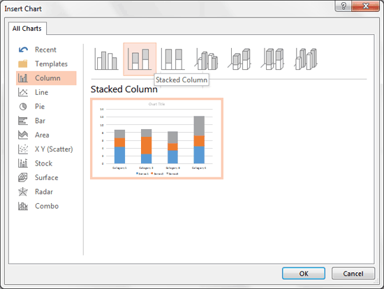
2. Selecting the Stacked Column chart: From within the Insert Chart dialog box, select the Stacked Column chart (this is what we will manipulate to create the Waterfall chart), which inserts the chart onto your slide and opens up an Excel spreadsheet.
3. 
   Figure 2: Select Stacked Column Chart

Which Stacked Column Chart?

Be sure to select the Stacked Column chart, and not the similarly-named 100% Stacked Column chart.

Setting up the Numbers

The most important step to building a Waterfall chart is setting up the numbers in Excel correctly. Throughout this tutorial, we will use the following data points to create the Waterfall Chart, as shown in Figure 3, below.

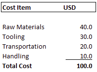
Figure 3: Data points to create the Waterfall Chart

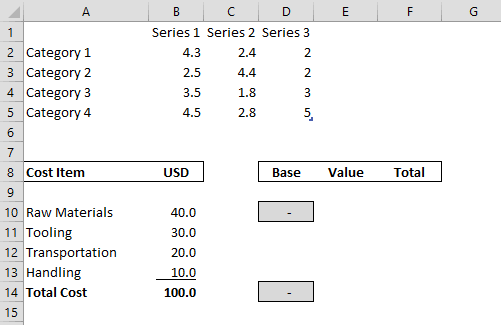
1. Prepping the Spreadsheet: With the above data inserted into the Excel spreadsheet starting at cell A8, the first step is to calculate the three data points we need for the Waterfall chart; what we will refer to as the Base, the Value, and the Total, as shown in Figure 4, below. We recommend always calculating them to the right of your original data points.
2. 
   Figure 4: Calculate the data points

Begin with a Base Value of Zero

We've formatted the first and last numbers in the Base column (D10 and D14) with a grey fill, and hardcoded the number 0 into each cell. Whenever building Waterfall Charts, the first, last, and any in-between sub-totals always need to start with a base value of zero.

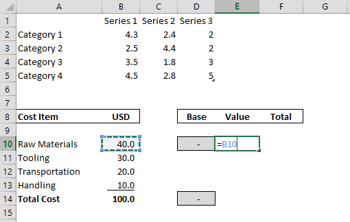
2. Calculating the Value: Let's continue with the first row of information for our Waterfall chart. We want to make the Value equal to our original number, so in cell E10, type in the formula "=B10", as shown in Figure 5, below.
3. 
   Figure 5: In cell E10, type in the formula "=B10"
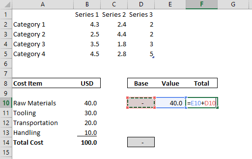
3. Calculating the Total: For the Total, we simply want to add up the Base and the Value. So in cell F10, type the formula "=E10 + D10", as shown in Figure 6, below.
4. 
   Figure 6: Adding the Base and the Value
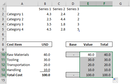
4. Filling in the Values and Totals: With the Value and Total calculated for the first row, we can then fill in the rest of the Values and Totals. So, selecting the first two cells, E10 and F10, copy the formula down to row 14. You can do this by selecting the small square in the lower right-hand corner and dragging it down to F14, as shown in Figure 7, below.
5. 
   Figure 7: Copy the formula down to row 14
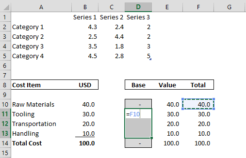
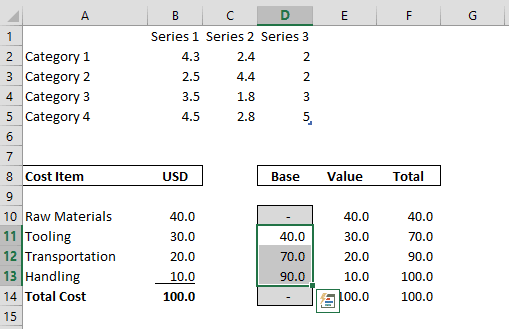
5. Calculating the 'Base': For the remaining Base numbers, we want to make them each equal to the previous data point's Total. So select cells D11 through D13, and type in the formula "=F10".
6. 
   Figure 8: Select cells D11 through D13
7. And then, holding the Ctrl key down, hit Enter, to input the formula into all of the selected cells, as shown in Figure 9, below.
8. 
   Figure 9: Hold Ctrl and hit Enter

Bringing the Information Into Our Chart, continued on Page 3 >